Differences of the builder pattern in Java and Python
In this post, we explore the differences in implementing the builder pattern in Java and Python.
1. Introduction
The builder design pattern 1, first introduced in the "Design Patterns: Elements of Reusable Object-Oriented Software" (1994) 2, popularly known as Gang of Four (GoF), is classified as a creational design pattern. This post focuses on its application in Java and Python.
At my current job we are using different programming languages. We decided to use the buildern pattern for one of our python microservices. While writing the buildern pattern in python, the team brought their "java style" to the python code. However, there is a pythonic way to write it and save some lines of code. This is the story behind this post.
2. Language features in Java and Python
Let's first examine the features of each language that we will later use to implement the design patterns in Python and Java. Python supports function default arguments 3 and named parameters 4, while Java supports function overloading 5.
The following examples demonstrates default arguments:
# Function with default arguments
def calculate_area(length, width=5):
    area = length * width
    print(f"Area: {area}")

# Using the function with both parameters
calculate_area(8, 4)

# Using the function with the default value for 'width'
calculate_area(10)  # Width defaults to 5

# You can still explicitly provide a value for 'width'
calculate_area(6, 3)
The following Python example demonstrates both default arguments and named parameters:
# Function with named parameters
def print_user_info(name, age, city="Unknown", country="Unknown"):
    print(f"Name: {name}, Age: {age}, City: {city}, Country: {country}")

# Using named parameters
print_user_info(name="John", age=25, city="New York", country="USA")

# Omitting some named parameters (using defaults)
print_user_info(name="Alice", age=30)

# Mixing ordered and named parameters
print_user_info("Bob", 28, country="Canada")
The following Java example shows how function overloading works:
// Java program to demonstrate working of method overloading in Java

public class Person {
    private String firstName;
    private String lastName;

    // Person constructor with two arguments, the first and last name.
    public Person(String firstName, String lastName) {
        this.firstName = firstName;
        this.lastName = lastName;
    }

    // Another constructor, this time with a single argument, the first name.
    public Person(String firstName) {
        this.firstName = firstName;
    }

    public static void main(String[] args) {
      // Using constructor with two parameters
      Person person1 = new Person("John", "Doe");
      // Using constructor with one parameter
      Person person2 = new Person("John");
  }
}
3. The builder pattern in Java 6
Factories and constructors share a limitation: they do not scale well to large numbers of optional parameters. Consider the case of a class representing the ingredients of a Pizza. Most ingredients have nonzero values for only a few of these optional fields.
What sort of constructors or static factories should you write for such a class? Traditionally, programmers have used the telescoping constructor pattern, in which you provide a constructor with only the required parameters, another with a single optional parameter, a third with two optional parameters, and so on, culminating in a constructor with all the optional parameters. Here’s how it looks in practice. For brevity’s sake, only three optional cheese fields are shown:
 1: public class Pizza {
 2:     private final int dough;      // 100g, 200g, 300g  required
 3:     private final int mozarella;  // 100g, 200g, 300g  optional
 4:     private final int parmesan;   // 50g, 100g, 150g   optional
 5:     private final int gorgonzola; // 50g, 100g, 150g   optional
 6:
 7:     public Pizza(int dough) {
 8:         this(dough, 0, 0, 0);
 9:     }
10:
11:     public Pizza(int dough, int mozarella) {
12:         this(dough, mozarella, 0, 0);
13:     }
14:
15:     public Pizza(int dough, int mozarella, int parmesan) {
16:         this(dough, mozarella, parmesan, 0);
17:     }
18:
19:     public Pizza(int dough, int mozarella, int parmesan, int gorgonzola) {
20:         this.dough = dough;
21:         this.mozarella = mozarella;
22:         this.parmesan = parmesan;
23:         this.gorgonzola = gorgonzola;
24:     }
25: }
When you want to create an instance, you use the constructor with the shortest parameter list containing all the parameters you want to set:
Pizza margarita = new Pizza(200, 200);
In short, the telescoping constructor pattern works, but it is hard to write client code when there are many parameters, and harder still to read it.
Luckily, the builder pattern helps us with the readability and tediousness of the code. Instead of making the desired object directly, the client calls a constructor with all of the required parameters and gets a builder object. Then the client calls setter-like methods on the builder object to set each optional parameter of interest. Finally, the client calls a parameterless build method to generate the object, which is typically immutable. The builder is typically a static member class of the class it builds. Here’s how it looks in practice:
public class Pizza {
    private final int dough;      // 100g, 200g, 300g  required
    private final int mozarella;  // 100g, 200g, 300g  optional
    private final int parmesan;   // 50g, 100g, 150g   optional
    private final int gorgonzola; // 50g, 100g, 150g   optional

    public static class Builder {
        // Required parameters
        private final int dough;

        // Optional parameters - initialized to default values
        private int mozarella = 0;
        private int parmesan = 0;
        private int gorgonzola = 0;

        public Builder(int dough) {
            this.dough = dough;
        }

        public Builder setMozarella(int val) {
            mozarella = val;
            return this;
        }

        public Pizza build() {
            return new Pizza(this);
        }
    }

    private Pizza(Builder builder) {
        dough = builder.dough;
        mozarella = builder.mozarella;
        parmesan = builder.parmesan;
        gorgonzola = builder.gorgonzola;
    }
}
The Pizza class is immutable, and all parameter default values are in one place. The builder’s setter methods return the builder itself so that invocations can be chained. Here’s how the client code looks:
Pizza pizza = new Pizza.Builder(200).setMozarella(200).setGorgonzola(50).build();
The Builder pattern simulates default arguments and named parameters as found in Python and eludes the telescoping pattern avoiding function overloading.
4. The builder pattern in Python
In python, we just simply leverage the language support for named parameters and default values as explained in 2 to write pythonic code for the builder pattern.
class Pizza:
    """
    Pizza class to represent a pizza with its ingredients.
    To set the ingredients the builder pattern is used.
    """

    def __init__(
        self,
        dough: int,
        mozarella: int = 0,
        parmesan: int = 0,
        gorgonzola: int = 0,
    ) -> None:
        self.dough = dough
        self.mozarella = mozarella
        self.parmesan = parmesan
        self.gorgonzola = gorgonzola
This time we do not need to concatenate calls, nor call a build method to instantiate a pizza object.
pizza = Pizza(200, mozarella=200, gorgonzola=50)
5. Summary
Exploring the Builder Pattern in Java and Python, we uncovered language-specific nuances. While Java employs an inner builder class to simulate features like named parameters and default arguments found natively in Python, the latter provides a more concise and idiomatic approach. The post contrasts these implementations, offering insights into the divergent paths each language takes when applying the Builder Pattern.
Footnotes:
Based on the excellent book "Effective Java: Programming Language Guide" (Third edition 2017) from Joshua Bloch. Item 2: Consider a builder when faced with many constructor paramters.
Java singleton
Not long time ago, I discovered in Java it is possible to implement a Singleton with an Enum. And not only that, it is the recommended way to implement them!
In this post, we explore the best practices when implementing the singleton pattern in Java.
1. Introduction
The following text is extracted from the wikipedia 1:
In software engineering, the singleton pattern is a software design pattern that restricts the instantiation of a class to a singular instance. One of the well-known "Gang of Four" design patterns 2, which describes how to solve recurring problems in object-oriented software, the pattern is useful when exactly one object is needed to coordinate actions across a system.
More specifically, the singleton pattern allows objects to:
- Ensure they only have one instance
- Provide easy access to that instance
- Control their instantiation (for example, hiding the constructors of a class)
The term comes from the mathematical concept of a singleton 3.
In this post, we'll dive into the best practices for implementing the singleton pattern in Java, considering key features such as concurrency, reflection, and serialization.
2. Java features to consider when creating a singleton
2.1. Concurrency
When creating a singleton in Java we need to make sure it is thread safe4. That is, when two or more threads instantiate a singleton only a single instance is created.
For this purpose, we will leverage the static keywork. The keyword static means that the particular member belongs to a type itself, rather than to an instance of that type.
From the java docs5: "If a field is declared static, there exists exactly one incarnation of the field, no matter how many instances (possibly zero) of the class may eventually be created.
2.2. Reflection
In the later examples, we will make use of a private contructor to implement the Singleton. With the help of Reflection6, an attacker could modify the runtime behaviour of the application modifying the accessibility of the private constructor to public. In other words, with the help of Reflection it would be possible to create a second instance of the class.
2.3. Serialization
Serialization is the process of translating an object into a format that can be stored or transmitted and reconstructed later. See figure 1.
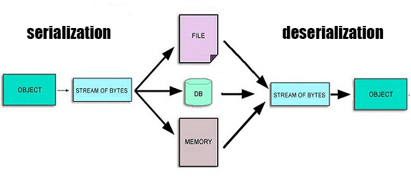
In Java, serializability of a class is enabled by the class implementing the java.io.Serializable interface.
Now, imagine your application serializes your singleton instance, so far so good, a stream of bytes has been created. However, when your application deserialize the same stream of bytes, it might end creating a new instance, leading, in the case of our example, to have two different instances!
Therefore we need to be carefull with Serialization when implementing our Singleton.
3. Singleton implementation
The two common ways of implementing singletons are based on keeping the constructor private and exporting a public static member to provide access to the instance.
In this first approach, the member INSTANCE is a final static field. The private constructor is called only once, to initialize the public static final field Spyderman.INSTANCE.
// Singleton with public final field
public class Spyderman {
    public static final Spyderman INSTANCE = new Spyderman();
    private Spyderman() { ... }
    public void withGreatPowerComesGreatResponsibility() { ... }
}
Thanks to the static final INSTANCE, we make sure the singleton is thread safe 2.1. However, an attacker could change thanks to reflection 2.2 the accessibility to the constructor, making it public or private and invoking it twice or more. We can defend ourselves against this attack making the constructor to throw an exception if it is invoked to create a second instance.
In the second approach to implement sigletons, the public member is a static method:
// Singleton with static factory
public class Spyderman {
    private static final Spyderman INSTANCE = new Spyderman();
    private Spyderman() { ... }
    public static Spyderman getInstance() { return INSTANCE; }
    public void withGreatPowerComesGreatResponsibility() { ... }
}
All calls to Spyderman.getInstance() return the same object reference. Same as the first example, it is thread safe thanks to the statics fields and it has the same caveat with reflection.
This second implementation is the prefered one, as it is more flexible, allowing the developer to remove the singleton property without changing the API as well as implement one singleton per thread or incorparating generics.
Now, if we need to make one of the above approaches Serializable adding implements Serializable, we need to modify our code to keep the singleton guarantee. Otherwise, each time a serialized instance is deserialized, as explained before 2.3, a new instance will be created. The solution would be to declare all instance fields transient and implement the readResolve method. We can find examples of this in the java.util.Collections7 file.
There is a third approach to the Singleton pattern, where we do not have to deal with thread safety, reflection nor serialization. It is the enum approach:
// Enum singleton - the preferred approach
public enum Spyderman {
    INSTANCE;
    public void withGreatPowerComesGreatResponsibility() { ... }
}
This approach look at first a bit inuntuituve. But lets check it properties. Every enum constant is always implicitly public static final which make it thread safe. There is no constructor that can be called by the developer so it makes it safe againts reflection attacks and as per documentation8 Enums are Serializable and special methods like readResolve are ignored.
The main disadvante is that Enums can not extend a superclass other than Enum, luckily, we can implement other interfaces.
4. Summary
We have seen why the Enum approach is often the best way to implement a singleton. The jvm provides the serialization and the protection against multiple instantiation and reflection attacks for free.
Footnotes:
Comparing Java map and Python dict
Recently, I have been asked how python solves hash collisions in
dictionaries. At that moment, I knew the answer for java maps, but
not for python dictionaries. That was the starting point of this entry.
Java maps and Python dictionaries are both implemented using hash tables,
which are highly efficient data structures for storing and retrieving
key-value pairs. Hash tables have an average search complexity of O(1),
making them more efficient than search trees or other table lookup
structures. For this reason, they are widely used in computer science.
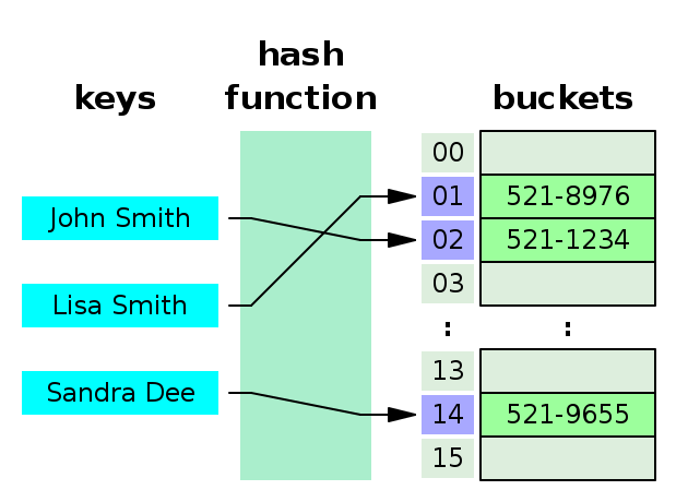
Figure 1 is a refresher of how hash tables works. Looking after a phone number in an agenda is a repetitive task, and we want it to be as fast as possible.
1. Hash collisions
Java maps and python dictionaries implementations differs from each other in how they solve hash collisions. A collision is when two keys share the same hash value. Hash collisions are inevitable, and two of the most common strategies of collision resolution are open addressing and separate chaining.
1.1. Separate chaining
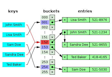
As shown in figure two, when two different keys point to the same cell value, the cell value contains a linked list with all the collisions. In this case the search average time is O(n) where n is the number of collisions. The worst case scenario is when the table has only one cell, then n is the length of your whole collection.
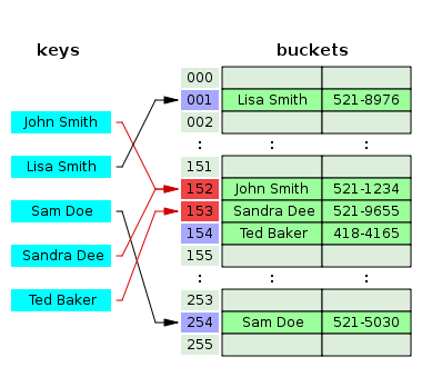
1.2. Open addressing
This technique is not as simple as separate chaining, but it should have a better performance. If a hash collision occurs, the table will be probed to move the record to a different cell that is empty. There are different probing techniques, for example in figure three the next cell position is used.
2. Java map
If we inspect the Hashmap class from the java.util package, we will see
that java uses separate chaining for solving hash clashes. Java also adds
a performance improvement, instead of using linked list to chain the
collisions, when there are too many collisions the linked list is
converted into a binary tree reducing the search average time from O(n)
to O(log2 n).
The code below correspond to the putVal method from the Hashmap
class which is in
charge of writing into the hash table. Line 6 writes into an empty
cell, line 17 inserts a new collision into a linked list and line 13
into a binary tree. Finally, line 19 converts the linked list into a
binary tree.
 1: final V putVal(int hash, K key, V value, boolean onlyIfAbsent, boolean evict) {
 2:     Node<K,V>[] tab; Node<K,V> p; int n, i;
 3:     if ((tab = table) == null || (n = tab.length) == 0)
 4:         n = (tab = resize()).length;
 5:     if ((p = tab[i = (n - 1) & hash]) == null)
 6:         tab[i] = newNode(hash, key, value, null);
 7:     else {
 8:         Node<K,V> e; K k;
 9:         if (p.hash == hash &&
10:             ((k = p.key) == key || (key != null && key.equals(k))))
11:             e = p;
12:         else if (p instanceof TreeNode)
13:             e = ((TreeNode<K,V>)p).putTreeVal(this, tab, hash, key, value);
14:         else {
15:             for (int binCount = 0; ; ++binCount) {
16:                 if ((e = p.next) == null) {
17:                     p.next = newNode(hash, key, value, null);
18:                     if (binCount >= TREEIFY_THRESHOLD - 1) // -1 for 1st
19:                         treeifyBin(tab, hash);
20:                     break;
21:                 }
22:                 if (e.hash == hash &&
23:                     ((k = e.key) == key || (key != null && key.equals(k))))
24:                     break;
25:                 p = e;
26:             }
27:         }
28:     }
29: }
The above code is extracted from the Java SE 17 (LTS) version, the binary tree improvement has been introduced in Java 8, in older versions the chaining was done only with linked lists.
3. Python dictionary
Python in contrast to java uses open addressing to resolve hash collisions. I recommend you to read the documentation from the source code: https://github.com/python/cpython/blob/3.11/Objects/dictobject.c Where the collision resolution is nicely explained at the beginning of the file.
Python resolves hash table collisions applying the formula
idx = (5 * idx + 1) % size, where idx is the table position.
Let's see an example:
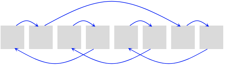
- Given a table of size
8 - We want to insert an element in position
0, which is not empty. - Applying the formula, the next cell to check is position
1[(5*0 + 1) % 8 = 1] - The cell is not empty, next try is position
6[(5*1 + 1) % 8 = 6] - The following try is position
7 [(5*6 + 1) % 8 = 7] - Next try is position
4 [(5*7 + 1) % 8 = 5] - Etc…
Can you spot the pattern?
Python adds some randomness to the process adding a perturb value which is
calculated with the low bits of the hash, the final formula is
idx = ((5 * idx) + 1 + perturb) % size.
Unfortunately, the C source code of CPython dictionaries is not as straight
forward as Java code is. This is due to some optimizations that we will
see later on, when we will talk about performance. We can see the formula
idx = ((5 * idx) + 1 + perturb) % size
in action in the method lookdict_index, where line 9 is an infinite
loop to find out the index, line 17 recalculates the perturb value and
line 18 applies the formula.
 1: /* Search index of hash table from offset of entry table */
 2: static Py_ssize_t
 3: lookdict_index(PyDictKeysObject *k, Py_hash_t hash, Py_ssize_t index)
 4: {
 5:     size_t mask = DK_MASK(k);
 6:     size_t perturb = (size_t)hash;
 7:     size_t i = (size_t)hash & mask;
 8:
 9:     for (;;) {
10:         Py_ssize_t ix = dictkeys_get_index(k, i);
11:         if (ix == index) {
12:             return i;
13:         }
14:         if (ix == DKIX_EMPTY) {
15:             return DKIX_EMPTY;
16:         }
17:         perturb >>= PERTURB_SHIFT;
18:         i = mask & (i*5 + perturb + 1);
19:     }
20:     Py_UNREACHABLE();
21: }
4. Performance
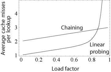
The above graph compares the average number of CPU cache misses required to look up elements in large hash tables with chaining and linear probing. Linear probing performs better due to better locality of reference, though as the table gets full, its performance degrades drastically.
Python uses dicts internally when it creates objects, functions, import modules, etc… Therefore, the performance of dictionaries is critical and linear probing is the way to go for them. The code below shows how python uses dictionaries internally when creating classes.
class Foo():
    def bar(x):
        return x+1

>>> print(Foo.__dict__)
{
  '__module__': '__main__',
  'bar': <function Foo.bar at 0x100d6b370>,
  '__dict__': <attribute '__dict__' of 'Foo' objects>,
  '__weakref__': <attribute '__weakref__' of 'Foo' objects>,
  '__doc__': None
}
4.1. Load factor
As we have seen the load factor is crucial for the performance of hash table, python has a load factor of 2/3 and java of 0.75. This makes sense, as linear probing performance is very bad when there are no empty hash spaces. On the other hand, java uses a threshold of 8 elements to switch from a linked list to a binary tree, as we can see in the code below.
static final float DEFAULT_LOAD_FACTOR = 0.75f;

/**
 * The bin count threshold for using a tree rather than list for a
 * bin. Bins are converted to trees when adding an element to a
 * bin with at least this many nodes. The value must be greater
 * than 2 and should be at least 8 to mesh with assumptions in
 * tree removal about conversion back to plain bins upon
 * shrinkage.
*/
static final int TREEIFY_THRESHOLD = 8;
5. What about sets
Dictionaries and maps are closely related to sets. In fact, sets are just dictionaries/maps without values. Indeed, Java uses this approach to implement sets, lets look at the source code:
/**
 * Constructs a new, empty set; the backing {@code HashMap} instance has
 * default initial capacity (16) and load factor (0.75).
 */
public HashSet() {
    map = new HashMap<>();
}
There are two different reasons why python does not reuse Objects/dictobject.c for implementing sets, the first one is that CPython does not use sets internally and the requirements are different. Looking after performance, CPython optimize the sets for the use case of membership. It is well documented in the source code to be found in Objects/setobject.c.:
/*
   Use cases for sets differ considerably from dictionaries where looked-up
   keys are more likely to be present.  In contrast, sets are primarily
   about membership testing where the presence of an element is not known in
   advance.  Accordingly, the set implementation needs to optimize for both
   the found and not-found case.
*/
A set is a different object and the hash table works a bit different, the set load factor is 60% instead of 66.6%, every time the table grows it uses a factor of 4 instead of 2, and the main difference is in the linear probing algorithm, where it inspects more than one cell for every probe.
6. Summary
CPython and Java use different approach to resolve hash collisions, while Java uses separate chaining, CPython uses linear probing. Java implements sets reusing hash tables but with dummy values, while python using also linear probing, optimizes the sets for different use cases, implementing a new linear probing algorithm. The reason for that is because CPython uses dictionaries internally and a high performance is critical for a proper performance of Python.
7. A note on source code
The source code examples are extracted respectively from the Java SE 17 (LTS) and CPython 3.11 versions.
